Modeling Stochastic Volatility a Review and Comparative Study

ane. Introduction

The paper explores the performance of Stochastic Volatility and GARCH(ane,1) models as estimators of the volatility of the S&P 500, the DOW JONES and the STOXX50 indices. The volatilities estimated by these models are compared with realized volatility estimates for the iii indices, obtained from the Oxford Man Realised Library, sampled at v-minute intervals, equally described in Heber et al. (2009). Their volatility forecasts are further compared with those derived from a uncomplicated historical volatility model. The data series features a 20 yr sample window of daily prices taken from 3 January 2000 to xxx April 2020, initially comprising 5100 observations, also taken from the Oxford Man Realised Library. The study is a companion written report to Allen and McAleer (2020).

The newspaper is motivated past Poon and Granger (2003, p. 507) who observed that: "as a rule of pollex, historical volatility methods work equally well compared with more sophisticated ARCH course and SV models." The paper features a continued exploration of this observation in the context of basic GARCH and Stochastic Volatility models equally compared with a simple historical volatility model based on lags of squared demeaned daily returns.

The R packages, stochvol and factorstochvol, are used, which employ Markov chain Monte Carlo (MCMC) samplers to conduct inference by obtaining draws from the posterior distribution of parameters and latent variables, which tin then be used for predicting future volatilities. This is done within the context of a fully Bayesian implementation of heteroskedasticity modelling within the framework of stochastic volatility. For more information, see the word of the methods by Kastner and Frühwirth-Schnatter (2014), Kastner et al. (2017), and of the stochvol and factorstochvol packages past Kastner (2016, 2019).

Taylor (1982) adult modelling volatility probabilistically, through a state-space model where the logarithm of the squared volatilities—the latent states—follow an autoregressive process of order i, which became known as the stochastic volatility (SV) model. Jacquier et al. (1994), Ghysels et al. (1996), and Kim et al. (1998) provided testify in support of the application of stochastic volatility models, but their applied use has been exceptional. The shortage of empirical applications of the SV models has been limited by 2 major factors: the variety (and potential incompatibility) of estimation methods for SV models, plus the lack of standard software packages (meet Bos (2012)). The situation for multivariate SV was even more problematic until Hosszejni and Kastner (2019) developed the R package 'factorstochvol'.

Taylor (1994) reviews the stochastic volatility and the ARCH/GARCH literature. Other reviews are past McAleer (2005) and Asai et al. (2006). Poon and Granger (2003, p. 485), noted the difficulties in the application of the SV model: "the SV model has no closed grade, and hence cannot be estimated straight by maximum likelihood". The advantage of the stochvol and factorstochvol R packages is that they incorporate an efficient MCMC interpretation scheme for SV models, as discussed by Kastner and Frühwirth-Schnatter (2014) and Kastner et al. (2017). These two R library packages facilitate the analysis in the newspaper, which features a direct comparison of the volatility predictions of a SV model, a GARCH (one,i) model, and a unproblematic application of a historical volatility based interpretation method, as applied to the the 3 indices.

The newspaper is divided into four sections: Section two reviews the literature and econometric method employed. Department iii presents the results, and Department 4 presents conclusions.

two. Previous Work and Econometric Models

ii.1. Stochastic Volatility

There accept been numerous empirical studies of changes in volatility in various stock, currency, and commodities markets. The findings in volatility inquiry have implications for pick pricing, volatility interpretation, and the degree to which volatility shocks persist. These research questions accept been approached past means of different models and methodologies.

Taylor (1982) suggested a novel SV arroyo, and Taylor (1994) developed the SV model every bit follows: if

$P_t$

denotes the prices of an asset at time

$t,$

and assuming no dividend payments, the returns on the asset can exist defined, in the context of discrete time periods, every bit:

$$X_t=ln[P_t/P_{t-1}].$$

(1)

Volatility is customarily indicated past

$\sigma$

, and prices are described past a stochastic differential equation:

$$d\left(lnP\right)=\mu dt+\sigma dW,$$

(2)

with West a standard Weiner procedure. If

$\mu$

and

$\sigma$

are constants,

${\mathrm{10}}_t$

has a normal distribution, and:

with

$U_t$

independent and identically distributed

$(i.i.d).$

Equation (iii) can be generalised by replacing

$\sigma$

with a positive random variable

${\sigma }_t$

, to give:

where

$U_t\sim N(0,\mathrm{i}).$

In circumstances where the returns process

$\left\{{\mathrm{10}}_t\right\}$

can be presented past Equation (4), Taylor (1994) calls

${\sigma }_t$

the stochastic volatility for menstruation t. His definition assumes that

$(X_t-\mu )/{\sigma }_t$

follows a normal distribution.

The stochastic process

$\left\{{\sigma }_t\right\}$

generates realised volatilities

$\left\{{\sigma }_t^{*}\right\}$

which, in full general, are not observable. For any realisation,

${\sigma }_t^{*}$

:

$$X_t\mid {\sigma }_t={\sigma }_{t^{*}}Ñ(\mu ,{\sigma }_{t^{*2}}).$$

(five)

The mixture of these provisional normal distributions defines the unconditional distribution of

${\mathrm{Ten}}_t$

, which volition have backlog kurtosis whenever

${\sigma }_t$

has positive variance and is contained of

$U_t$

.

In the empirical section which follows, I use the RV of the S&P500, DOW JONES and STOXX50 indices, sampled at 5-minute intervals provided past Oxford Man, as a proxy for the true realised volatility. I and then compare the estimates of volatility obtained from SV and GARCH(1,1) models, using the RV estimates as a criterion.

Taylor (1994, p. iii) suggests using "majuscule letters to represent random variables and lower case letters to stand for outcomes". I shall follow that convention. Given observed returns of

$I_{t-1}=\{x_1,x_2,.....{\mathrm{ten}}_{t-\mathrm{i}}\}$

the provisional variance for period t is:

$$h_t=var(X_t\mid I_{t-1}).$$

(half-dozen)

Taylor (1994) notes that, in general, the random variable

$H_t$

, which generates the observed provisional variance

$h_t$

is not, in general, equal to

${\sigma }_t^{\mathrm{two}}$

. A convenient way to utilize economic theory to motivate changes in volatility is to assume that returns are generated by a number of intra-menstruation price revisions, as in the manner of Clark (1973) and Tauchen and Pitts (1983).

It is assumed that there are

$N_t$

cost revisions during trading day t, each caused past unpredictable information. Allow issue i on day t change the logarithmic price by

${\omega }_{it}$

, with:

$$X_t=\mu +\sum _{i=1}^{{\mathrm{Northward}}_t}{\omega }_{it}.$$

(seven)

If we assume that

${\omega }_{it}\sim$ $i.i.d.$

and is independent of the random variable

$N_t$

, with

${\omega }_{it}\sim \mathrm{Northward}(0,{\sigma }_{\omega }^2)$

, then:

$${\sigma }_t^{\mathrm{ii}}={\sigma }_{\omega }^2{\mathrm{Due\; north}}_{t}a\mathrm{northward}d{H}_t={\sigma }_{\omega }^2\mathrm{Due\; east}[N_t\mid I_{t-\mathrm{ane}}].$$

(8)

The higher up model suggests that squared volatility is proportional to the corporeality of price information.

The lack of standard software to estimate such a model is addressed by Kastner and Frühwirth-Schnatter (2014) who propose an efficient MCMC interpretation scheme which is implemented in the R stochvol package, Kastner (2016). Kastner (2016, p. 2) proceeds by "letting

$y={(y_{\mathrm{one}},y_2,.....y_n)}^{|}$

be a vector of returns, with hateful zero. An intrinsic feature of the SV model is that each observation

$y_t$

is assumed to have its 'own' contemporaneous variance,

${\mathrm{east}}^{h_t}$

, which relaxes the usual assumption of homoscedasticity". Information technology is assumed that the logarithm of this variance follows an autoregressive process of lodge i. This assumption is fundamentally different to GARCH models, where the time-varying conditional volatility is assumed to follow a deterministic instead of a stochastic evolution.

The centered parameterization of the SV model tin be given equally:

$$y_t\mid h_t\sim N(0,\mathrm{due\; east}xp{}^{h_t}),$$

(9)

$$h_t\mid h_{t-1},\mu ,\varphi ,{\sigma }_n\sim \mathrm{North}(\mu ,+\varphi (h_{t-1}-\mu ),{\sigma }_{\mathrm{due\; north}}^{\mathrm{two}}),$$

(x)

$$h_0\mid \mu ,\varphi ,{\sigma }_{\mathrm{north}}\sim N(\mu ,{\sigma }_n^2/(1-{\varphi }^{\mathrm{ii}}),$$

(11)

where

$N(\mu ,{\sigma }_{\mathrm{north}}^2)$

denotes the normal distribution with mean

$\mu$

and variance

${\sigma }_n^2$

.

$\theta ={(\mu ,\varphi ,{\sigma }_n)}^{|}$

is the vector of parameters which consists of the level of the log variance

$\mu$

, the persistence of log variance,

$\varphi$

, and the volatility of log variance,

${\sigma }_n.$

The process

$h={(h_0,h_1,......,h_{\mathrm{northward}})}^{|}$

which features in equations (x) and (11) is the unobserved or latent time-varying volatility process.

Kastner (2016, p. four) remarks that: "A novel and crucial feature of the algorithm implemented in stochvol is the usage of a variant of the "ancillarity-sufficiency interweaving strategy" (ASIS) which was suggested in the general context of state-space models by Yu and Meng (2011). ASIS exploits the fact that, for certain parameter constellations, sampling efficiency improves substantially when considering a non-centered version of a country-space model".

Another key feature of the algorithm used in stochvol is the articulation sampling of all instantaneous volatilities "all without a loop" (AWOL), a technique with links to Rue (2001) and as discussed in McCausland et al. (2011). The combination of these features enables the R parcel stochvol to approximate SV models efficiently even when large datasets are involved.

Kastner et al. (2017) propose that the multivariate factor stochastic volatility (SV) model (Chib et al. 2006) provides a ways of uniting simplicity with flexibility and robustness. Information technology is simple in the sense that the potentially high-dimensional observation space is reduced to a lower-dimensional orthogonal latent factor space. It is flexible in the sense that these factors are immune to exhibit volatility clustering, and it is robust in the sense that idiosyncratic deviations are themselves stochastic volatility processes, thereby allowing for the degree of volatility co-movement to be fourth dimension-varying. Hosszejni and Kastner (2019) fix upward a cistron SV model employed in the factorstochvol package in R, and the analysis also uses code from this package.

two.2. Curvation and GARCH

Engle (1982) developed the Autoregressive Conditional Heteroskedasticity (Curvation) model that incorporates all by error terms. It was generalised to GARCH by Bollerslev (1986) to include lagged term provisional volatility. GARCH predicts that the best indicator of future variance is a weighted average of long-run variance, the predicted variance for the current period, and whatsoever new information in this period, every bit captured by the squared residuals.

Consider a time series

$y_t=E_{t-1}\left(y_t\right)+{\epsilon }_t,$

where

$E_{t-1}\left(y_t\right)$

is the provisional expectation of

$y_t$

at fourth dimension

$t-1$

and

${\epsilon }_t$

is the error term. The basic GARCH model has the post-obit specification:

$${\epsilon }_t=\sqrt{h_t{\eta }_t}{\eta }_t(0,1)$$

(12)

$$h_t=\omega +{\displaystyle \sum _{j=1}^p}{\alpha }_j{\epsilon }_{t-j}^2+\sum _{j=\mathrm{ane}}^q{\beta }_j{h}_{t-j}$$

(13)

in which

$\omega >0,{\alpha }_j\ge 0$

and

${\beta }_j\ge 0$

(usually a positive fraction), to ensure a positive conditional variance,

$h_t\ge 0$

(run across Tsay (1987)). The ARCH event is captured by the parameter

${\alpha }_j,$

which represents the short-run persistence of shocks to returns,

${\beta }_j$

captures the GARCH effect that contributes to long-run persistence, and

${\alpha }_j+{\beta }_j$

measures the persistence of the affect of shocks to returns to long-run persistence. A GARCH(1,one) process is weakly stationary if

${\alpha }_j+{\beta }_j\le 1$

. (See the discussion in Allen et al. (2013).

We contrast the estimates of volatility from the SV model with those from a GARCH(1,one) model, and assess which better explains the behaviour of the RV of FTSE sampled at 5-minute intervals.

two.iii. Realised Volatility

Use was made of the RV five-min estimates from Oxford Man for the iii indices as the RV criterion (see: https://realized.oxford-human being.ox.ac.uk/data). This database contains "daily (close to close) financial returns, and a corresponding sequence of daily realised measures

$r{\mathrm{one\; thousand}}_1,r{m}_2,.....,r{m}_T$

. Realised measures are theoretically audio loftier frequency, nonparametric-based estimators of the variation of the price path of an asset during the times at which the asset trades often on an exchange. Realised measures ignore the variation of prices overnight and sometimes the variation in the get-go few minutes of the trading day when recorded prices may contain large errors". The metrics were developed by Andersen et al. (2001), Andersen et al. (2003), and Barndorff-Nielsen and Shephard (2002). Shephard and Sheppard (2010) provide an business relationship of the RV measures used in the Oxford Man Realised Library.

The simplest realised metric is realised variance (RV):

$$R{V}_t=\sum x_{j,t}^{\mathrm{two}},$$

(fourteen)

where

$x_{j,t}=X_{t_{j,t}}-X_{t_{j-\mathrm{ane},t}}$

. The

$t_{j,t}$

are the times of trades or quotes on the t-th day. The theoretical justification of this measure is that, if prices are observed without noise so, as

$\mathrm{grand}inj\mid t_{j,t}-t_{j-\mathrm{ane},t}\mid \downarrow 0$

, information technology consistently estimates the quadratic variation of the price process on the t-thursday twenty-four hours. If the sampling is reduced to very small intervals of fourth dimension, market microstructure dissonance may become a contaminant. In order to avoid this upshot, we use RV estimates from Oxford Man, sampled at 5-infinitesimal intervals, hereafter

$RV\mathrm{v}.$

2.4. Historical Volatility Model

Poon and Granger (2005) hash out diverse applied bug involved in forecasting volatility. They suggest that the HISVOL model has the following form:

$${\widehat{\sigma }}_t={\varphi }_1{\sigma }_{t-\mathrm{ane}}+{\varphi }_2{\sigma }_{t-\mathrm{two}}+..+{\varphi }_{\tau }{\sigma }_{t-\tau },$$

(15)

where

${\widehat{\sigma }}_t$

is the expected standard divergence at time t,

$\varphi$

is the weight parameter, and

$\sigma$

is the historical standard deviation for periods indicated by the subscripts. Poon and Granger (2005) propose that this group of models include the random walk, historical averages, autoregressive (fractionally integrated) moving average, and diverse forms of exponential smoothing that depend on the weight parameter

$\varphi$

.

We utilise a simple form of this model in which the judge of

$\sigma$

is the previous 24-hour interval'south demeaned squared render. Poon and Granger (2005) review 66 previous studies, and suggest that implied standard deviations announced to perform all-time, followed by historical volatility and GARCH which have roughly equal performance. They also note that, at the time of writing, there were insufficient studies of SV models to come up to any conclusions about this class of models. This ascertainment provides the motivation for the current study which assesses the operation of all 3 classes of models. It as well provides the motivation to utilise a crude rule of thumb in the form of 20 lags of daily squared demeaned returns. The selection of twenty lags is conditioned by Corsi's (2009) "Heterogeneous Autoregressive model of Realized Volatility" (HAR) model, as discussed in the next department. A feature of this model is that it includes estimates of daily, weekly, and monthly ex-post realised volatility. The crude HISVOL model adopted in the paper takes 20 lags as an approximation for this, as it roughly represents a month of trading days.

Barndorff-Nielsen and Shephard (2003) point out that taking the sums of squares of increments of log-prices has a long tradition in the financial economics literature. Come across, for case, Poterba and Summers (1986), Schwert (1989), Taylor and Xu (1997), Christensen and Prabhala (1998), Dacorogna et al. (1998), and Andersen et al. (2001). (Shephard and Sheppard (2010), p 200, footnote 4) note that: "Of form, the well-nigh bones realised measure is the squared daily return". We utilise this arroyo as the basis of our historical volatility model.

2.5. Heterogenous Autoregressive Model (HAR)

Corsi (2009, p. 174) suggests "an additive cascade model of volatility components divers over different time periods. The volatility cascade leads to a simple AR-type model in the realized volatility with the feature of considering dissimilar volatility components realized over different fourth dimension horizons and which he termed every bit a "Heterogeneous Autoregressive model of Realized Volatility". Corsi (2009) suggests that the model successfully achieves the purpose of reproducing the master empirical features of financial returns (long retentivity, fatty tails, and self-similarity) in a parsimonious way. He writes his model every bit:

$${\sigma }_{t+1d}^{\left(d\right)}=c+{\beta }^{\left(d\right)}R{\mathrm{Five}}_t^{\left(d\right)}+{\beta }^{\left(\mathrm{due\; west}\right)}R{\mathrm{Five}}_t^{\left(\mathrm{due\; west}\right)}+{\beta }^{\left(\mathrm{chiliad}\right)}R{V}_t^{\left(\mathrm{thousand}\right)}+{\tilde{\omega }}_{t+1d}^{\left(d\right)},$$

(16)

where

${\sigma }^{\left(d\right)}$

is the daily integrated volatility, and

$R{\mathrm{Five}}_t^{\left(d\right)},$ $R{\mathrm{Five}}_t^{\left(w\right)}$

and

$R{V}_t^{\left(\mathrm{one\; thousand}\right)}$

are respectively the daily, weekly, and monthly (ex mail service) observed realized volatilities, and

${\mathrm{due\; west}}_{t+1d}={\tilde{\omega }}_{t+1d}^{\left(d\right)}-{\omega }_{t+\mathrm{ane}d}^{\left(d\right)}$

.

Corsi (2009) inspires the HISVOL model adopted in the paper, which uses lags of historical RV estimates, but, in the current case, lags of squared demeaned daily close-to-shut returns are employed.

A further justification for the approach adopted in the current study is provided by a contempo publication by Perron and Shi (2020), who prove that squared low-frequency daily returns tin can be expressed in terms of the temporal assemblage of a high-frequency series. They explore the links between the spectral density function of squared low-frequency and high-frequency returns. They analyze the properties of the spectral density function of realized volatility, constructed from squared returns with different frequencies nether temporal aggregation. Even so, for the low frequency information on S&P 500 returns, they cannot infer whether the noise is stationary long memory but a long-memory process appears needed to explain the features related to loftier frequency S&P 500 futures. However, they caution that they cannot explain this difference and that information technology may also be related to the fact that they have used both spot and futures serial for the S&P500 in the case of the high frequency data.

Perron and Shi (2020, p. 14), advise that: "that both the realized volatility and the squared daily returns comprise the same information about long memory. However, the squared daily returns contain a larger dissonance component than does the realized volatility". The current paper uses the long-memory component of low frequency squared daily demeaned returns to capture this long memory feature and to provide an approximation to a HAR model. The paper does not apply a full HAR model every bit the intention is to explore whether a simple HISVOL rule of thumb model, based on lagged squared demeaned returns, performs as well as standard GARCH or SV models. Information technology is clear that a total HAR specification is probable to perform improve, though Perron and Shi (2020) suggest that many of the HAR's long retentivity features will be captured past the approach adopted in the paper.

3. Results of the Analysis

three.1. Preliminary Analysis

The sample information set consists of 20 years and four months of daily data of adjusted continuously compounded close to close returns for S&P 500, DOW JONES and STOXX50 indices, taken from 3 Jan 2000 through to thirty April 2020. There are a matching set of daily RV5 estimates for the three indices obtained from the Oxford Human Realised library. These 3 indices are called considering they plant major components of global capital markets in the US and in Europe.

The S&P500 reflects the performance of the top 500 stocks of leading companies in the Usa, and is listed on the NYSE (New York Stock Exchange) and (Nasdaq Exchange). The companies included comprise roughly 80% coverage of the bachelor United states market capitalisation. The DOW JONES index is a much narrower alphabetize that measures the daily price movements of 30 big American companies on the Nasdaq and the New York Stock Substitution and is comprised of baddest stocks. The EURO STOXX fifty is a stock index of Eurozone stocks designed by STOXX, an index provider owned by Deutsche Börse Group. STOXX suggests that the aim is "to provide a blue-fleck representation of Supersector leaders in the Eurozone". It is fabricated up of fifty of the largest and nearly liquid stocks. These indices are representative of blue chip stocks in the Usa and Eurozone, plus the broader U.s. market. Thus, these indices are likely to be of great importance and appeal to investors given the nature of the markets that they cover.

Summary statistics for the six serial are provided in Table 1. The sample size varies for the iii indices varies given a dissimilar incidence of holidays in the Us and in Europe. For case, in 2019, at that place were 9 days of vacation related closures on the NYSE but just five in Europe. The total number of sample observations for the USA indices initially comprised 5100 data points whilst the full for the STOXX50 was 5180.

Close to close returns were used because it was thought that these are likely to capture all the information released over a 24 h period and would provide more accurate measures of volatility for the demeaned squared return series used in the regression tests.

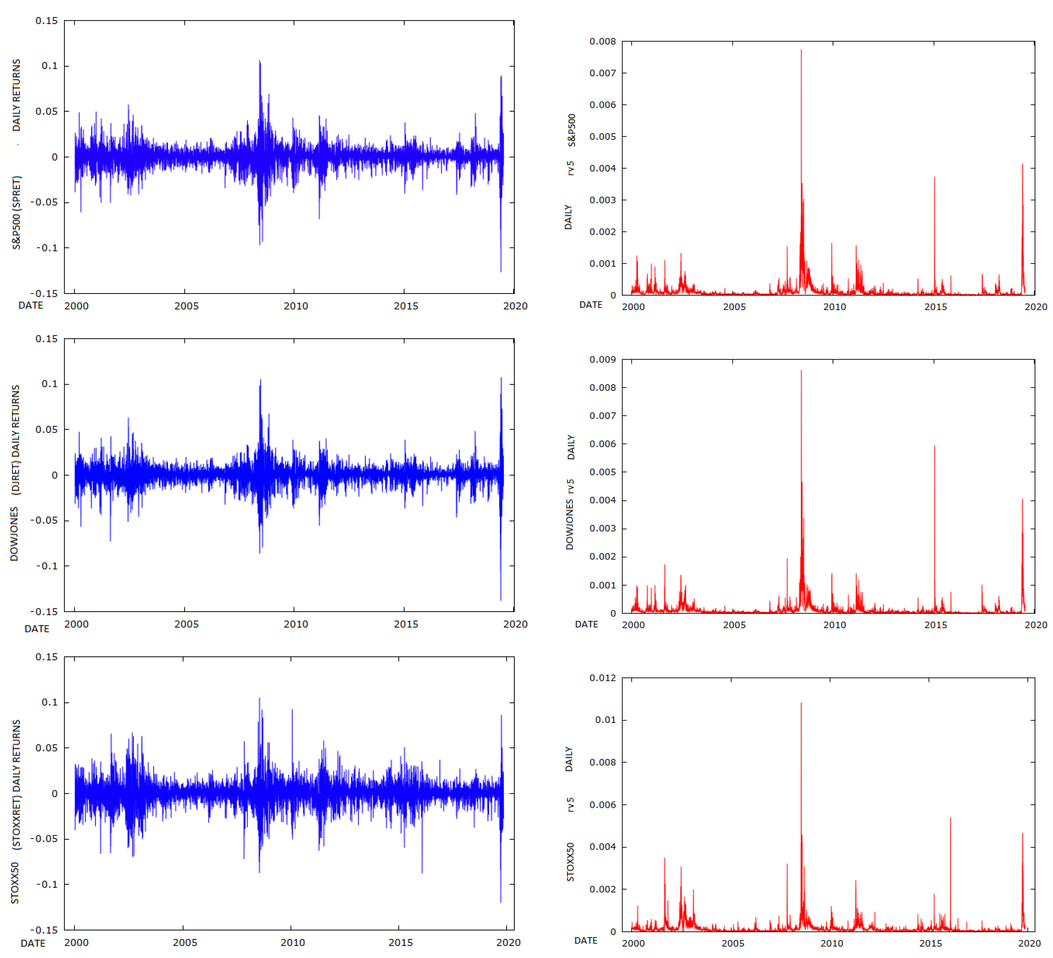
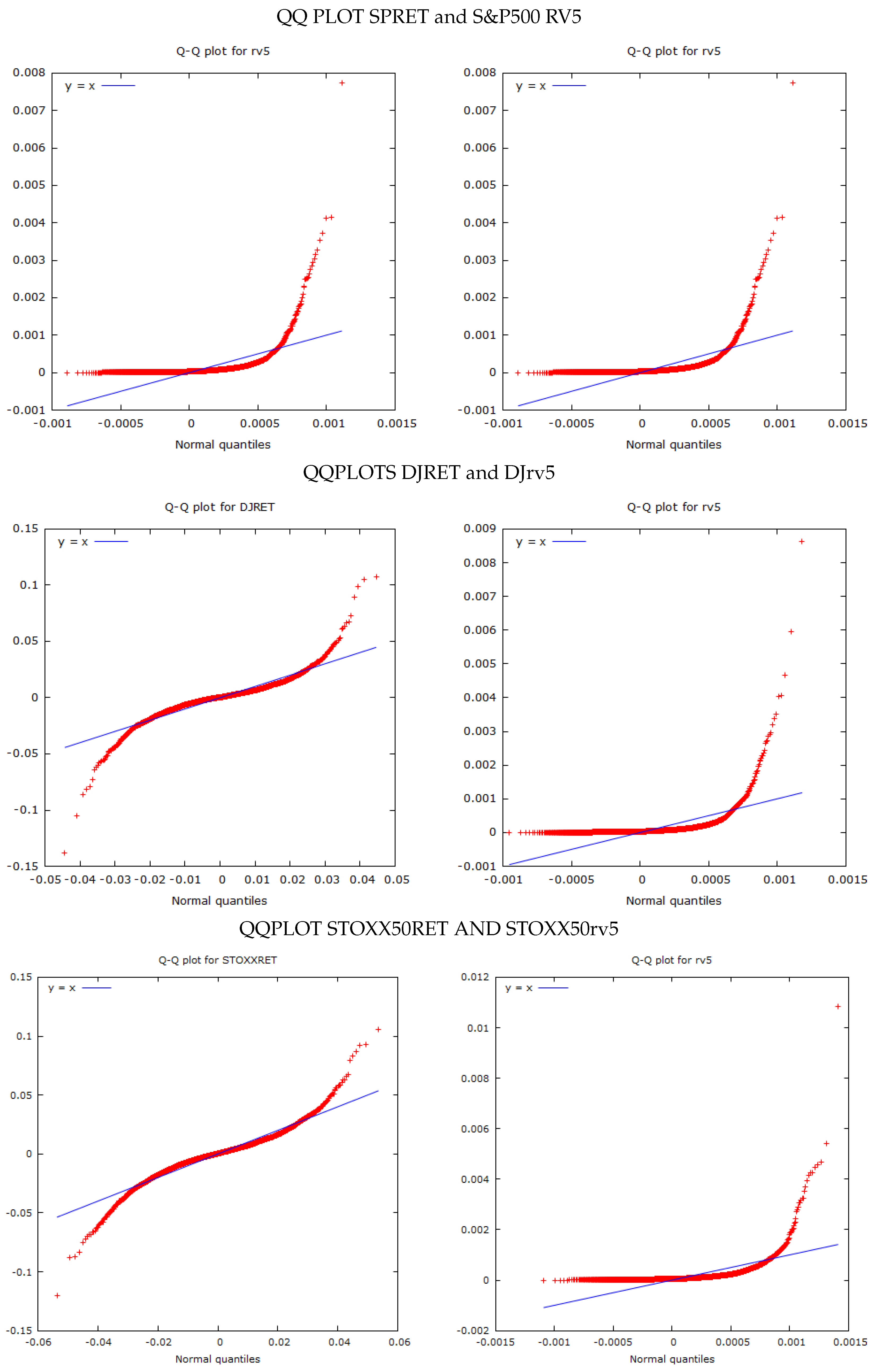
The S&P500 has a hateful daily return of 0.01361 per cent and a standard deviation of one.248 per cent. Plots of the daily returns and RV5 estimates are provided in Figure i. Information technology had positive excess kurtosis and does not adjust to a Gaussian distribution, as can exist seen from the QQ plot in Figure 2. The Southward&P500 RV5 has a mean of 0.00011202 and a standard divergence of 0.00026873. Withal, Rv5 is measured as a variance, and, if we take the square root of its value and multiply it past 100, it will be on a mutual scale with the Southward&P500 returns. Nosotros undertake this transformation in some of the comparison plots in subsequent figures. It has very high skewness and kurtosis which is too evident in the QQ plots in Figure ii.

The DOWJONES has a hateful return of 0.01496 per cent and a standard deviation of 1.1946 per cent, while STOXX50 has a mean return of −0.0098108 per cent and a standard deviation of one.4439. DOWJONES RV5 has a hateful of 0.00011386 and a standard deviation of 0.00028661, while RV5 of DOWJONES has a hateful of 0.00011386 and a standard divergence of 0.00028661. STOXX50 RV5 has a mean of 0.00016066 and a standard deviation of 0.00033556. All iii RV5 series are skewed and take loftier excess kurtosis.

iii.2. SV and GARCH Estimates

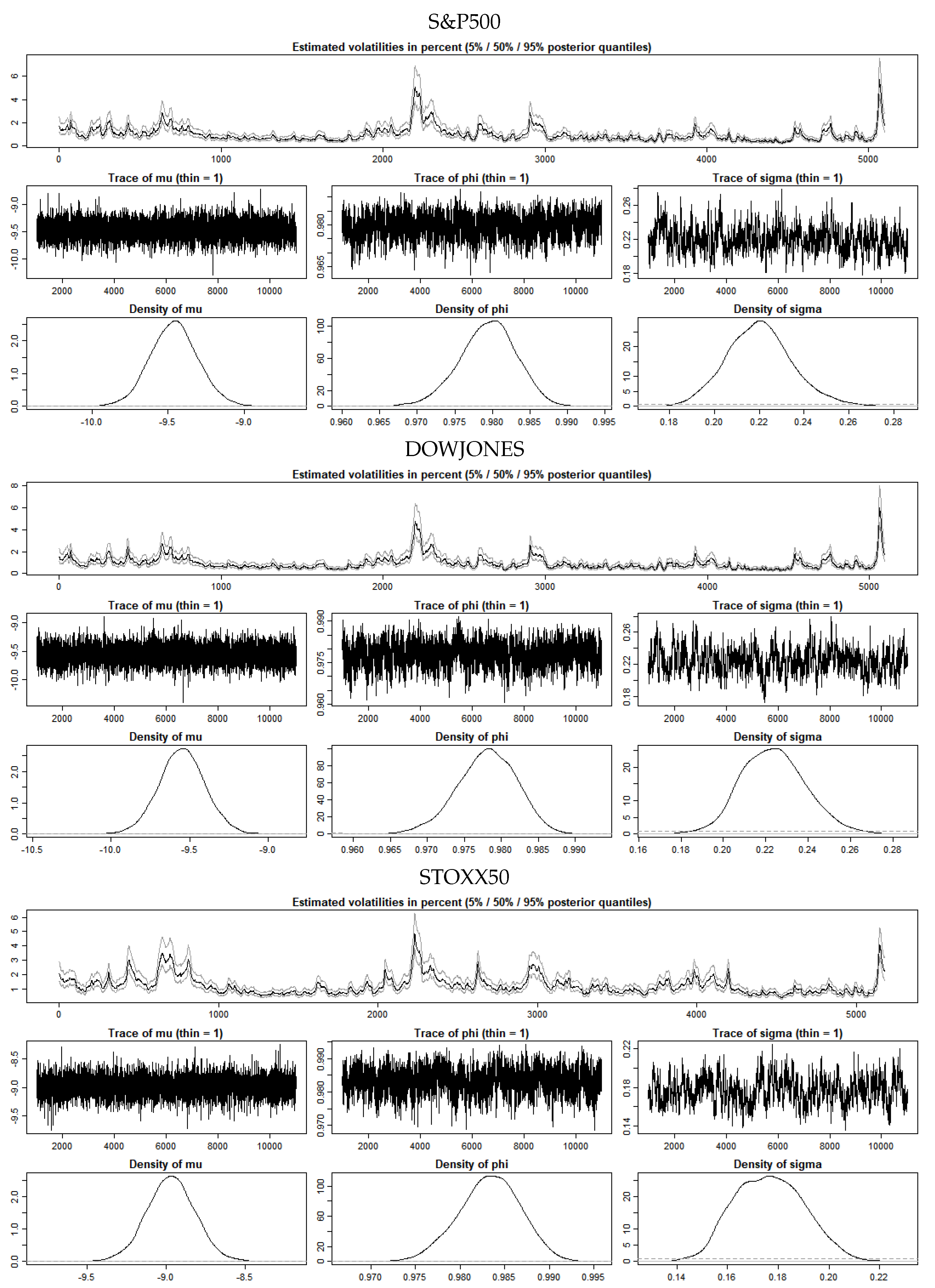
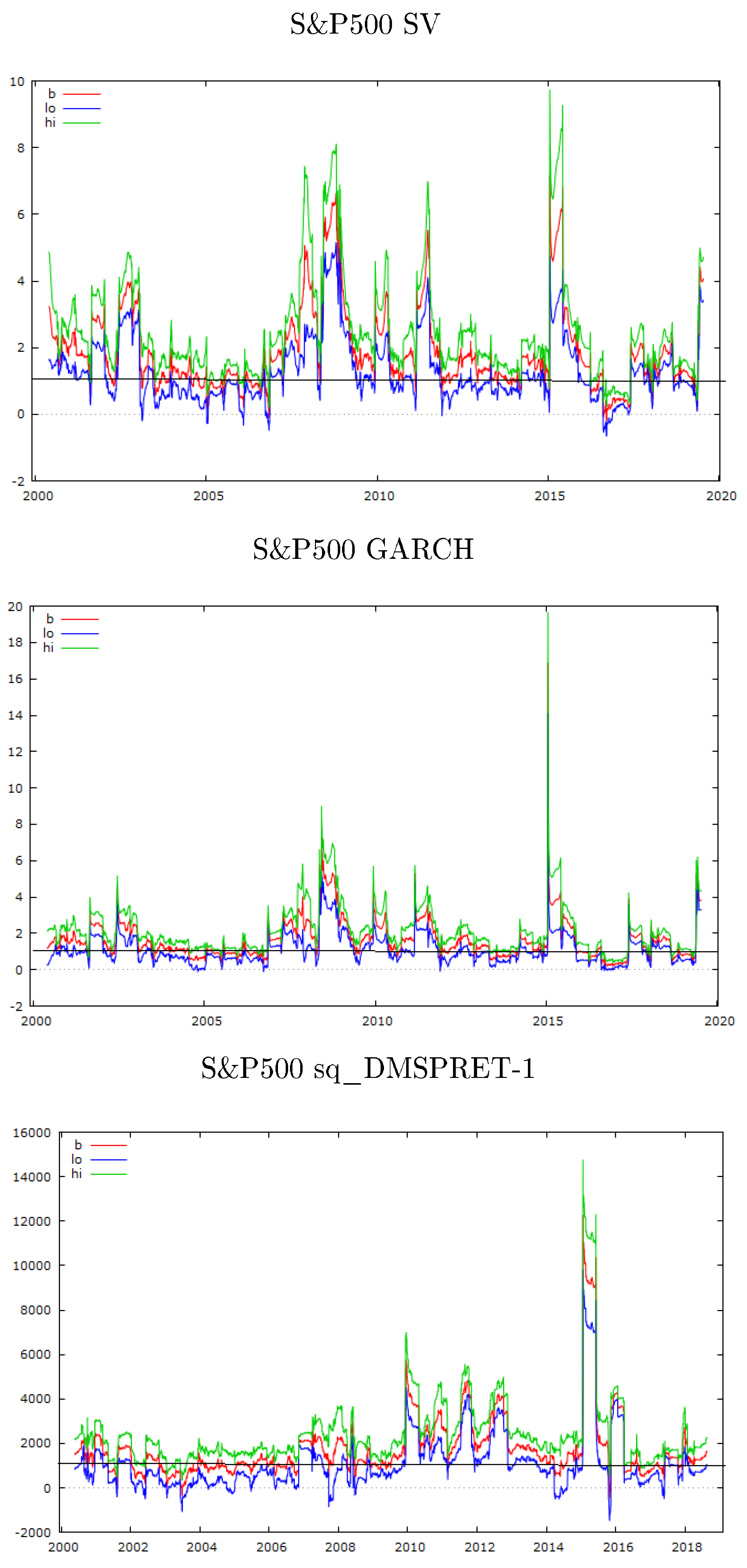
The R library stochvol was used to fit a stochastic volatility model to the South&P500, DOWJONES and STOXX50 de-meaned return serial, and Gaussian distributions applied to fit the SV model. Some of the initial parameters for the SV model estimation, as applied to the three series, are shown in Tabular array 2. The SV model practical to the three serial produces the volatility estimates shown in Figure 3, while Figure 4 displays a comparison of the volatility estimates for both a GARCH (1,1) model and the SV model, as applied to the three return series. The estimates of volatility are quite similar. The estimates for the GARCH(one,i) model used to obtain provisional volatilities are shown in Table 3. The diagnostic tests (not reported), suggested that the models are a satisfactory fit and that the volatility model parameter estimates are within stable limits.

The benchmark used in this paper is the same as in Allen and McAleer (2020), namely estimates of realised volatility sampled at five-infinitesimal intervals, as obtained from Oxford Human. These are employed as the baseline in ordinary least squares regressions adopted to explore the linear correlations betwixt the estimates of the two volatility models and the base RV5 estimates of volatility. The results are shown in panels A, B and C of Tabular array four.

All the regressions reported in Table 4 utilise RV5 values as the criterion dependent variable, for the three index serial. The offset set of regressions in each panel reports the results of the regression of RV5 on the predictions of volatility obtained from the SV model, lagged by one solar day. Each of the iii estimated coefficients on SV, for the three indices South&P500, DOW JONES and STOXX50, with respective values of 0.000305766, 0.000328020 and 0.000249773 are significant at the 1 per cent level. The respective adjusted R-Squares of these regressions are 0.528418, 0.483024 and 0.398682. The results suggest that the base SV model captures between 40 and l per cent of the volatilities of the iii index series when the benchmark is RV5.

As a further cantankerous-bank check of the effectiveness of the two models, we used a farther crude estimate of volatility with the demeaned squared daily returns on the three serial, in the context of a HISVOL model, which is motivated by Corsi's (2009) Heterogeneous Autoregressive model of Realized Volatility (HAR-RV).

This rough model produces better results than those using SV and GARCH(1,1) provisional volatilities equally explanatory variables. The adjusted R-squared values are 0.540166 for the Due south&P500 Index in Panel A, 0.445781 in Console B for DOWJONES, and 0.443043 in Panel C for STOXX50. The adjusted R-square values obtained by this crude approximation to a HAR-RV model all exceed the explanatory values produced by the SV and GARCH(1,one) models in two of the three cases with the exception of the DOWJONES. These results are largely consistent with Allen and McAleer (2020).

iii.3. Mincer–Zarnowitz Tests

As an additional test of the accuracy of the forecasts, I used some Mincer and Zarnowitz (1969) regression tests. (I am grateful to a reviewer for this proffer). The test involves regressing realised values on the forecasts:

$${\sigma }_{t+1}={\beta }_0+{\beta }_{\mathrm{ane}}{\widehat{\sigma }}_{t+1}.$$

The joint hypothesis tested is that

${\beta }_0=0,$

and

${\beta }_{\mathrm{i}}=\mathrm{i}.$

The results of the test on the full sample are shown in Tabular array 5.

The results in Table five uniformly and significantly reject the accuracy of the forecasts. However, the forecasts involve long time series with in excess of 5000 observations. As a farther check, I ran some rolling Mincer–Zarnowitz regressions using a 100 observation window to explore how frequently the slope coefficient had a value of ane bounded within two standard deviation intervals. This was done to check the relative frequency of periods in which the forecasts could not reject the zippo hypothesis. The results for the S&P500 index are shown in Effigy 5 (I have omitted the results of the other series in the interests of brevity, merely they are available from the author on asking).

It tin exist seen in Figure five that there are extended periods of time in which the cipher hypothesis that the slope coefficient of the results of regressing the bodily on the forecast is not significantly different from 1. This highlights the problems related to type one and type two errors. It also is consistent with the Mincer–Zarnowitz tests consistently rejecting the null hypothesis yet the adjusted Rsquares of the regressions of actuals on forecasts being consistently in the range of 40–50%.

3.4. Further Assay

Kastner (2019) in the factorstochvol R bundle, together with the Hosszejni and Kastner (2019) vignette, on factorstochvol, demonstrated how to expand the capabilities of the original stochvol bundle. In particular, they explained how it is possible to construct a multiple regression model with an intercept, 2 regressors, and SVl residuals using the following construction:

$$\left(\begin{array}{c}{y}_t\\ h_{t+\mathrm{one}}\end{array}\right)\mid h_t,\varsigma ,\left(\begin{array}{c}{x}_{t1}\\ x_{t2}\end{array}\right),{\beta }_0,\left(\begin{array}{c}{\beta }_1\\ {\beta }_{\mathrm{ii}}\end{array}\right)~N_2\left(\left(\begin{array}{c}{\beta }_0+{\beta }_1{x}_{t1}+{\beta }_2{\mathrm{10}}_{t\mathrm{ii}}\\ u+\phi (h_t-\mu )\end{array}\right),{{\displaystyle \sum }}^{\rho }\right),$$

(17)

$${\displaystyle {\sum }^{\rho }}=\left(\begin{array}{cc}{\displaystyle \mathrm{due\; east}xp\left(h_t\right)}& {\displaystyle \rho \sigma \mathrm{due\; east}\mathrm{10}p(h_t/2)}\\ {\displaystyle \rho \sigma e\mathrm{10}p(h_t/2)}& {\displaystyle {\sigma }^{\mathrm{ii}}}\end{array}\right).$$

This arroyo was adopted to include the second and tertiary moments of the alphabetize series in the form of de-meaned squared returns and de-meaned cubed returns as the two regressors in the regression model. The intention was to check whether these simple enhancements would improve the operation of the basic stochastic volatility model, in regression tests which used the estimated volatility, every bit reported in the previous section, as the explanatory variable regressed on the benchmark values of RV5 for the iii index series. Table 6 presents the the stochastic volatility estimates for the augmented model and posterior density plots of parameters in

$\theta$

are shown in Effigy half dozen.

The values appear to exist reasonably well-behaved and the density plots in Figure half-dozen are adequate, although the density estimates for the STOXX50 are the weakest of the three with some bear witness of bimodality in the mu estimation plot.

A similar simple enhancement was practical to the GARCH(1,1) conditional volatility model in which the mean equation featured the addition of a vector of squared de-meaned returns to assess whether this improved its explanatory operation. The results of the GARCH(1,i) models with enhanced mean equations are not reported in the newspaper in the interests of brevity, only are available on asking. Suffice to say all the estimates appeared to be satisfactory.

Tabular array vii reports the results of the regression analyses featuring the volatility estimates from both the augmented stochastic volatility and GARCH models. The results are mixed. The benchmark in Table 4 is provided past the 'rule of thumb' historical volatility model in which 20 lags of de-meaned shut-to-close returns were regressed on the Oxford Human RV5 estimates for the three indices. The adjusted R-squares in the cases of the Southward&P500, DOWJONES and STOXX50 were, respectively, 0.54, 0.54, and 0.44. The augmented SV model for the Southward&P500, as shown in the first regression in Table six, has an adjusted R-square of 0.56, a marginal improvement. The original GARCH model for this index had an adjusted R-square of 0.36, which also improves marginally to 0.37.

The DOWJONES historical volatility model'due south adapted R-square of 0.54 is not matched by that for the augmented SV model, which is 0.43 in Table vii. Notwithstanding, the adjusted R-foursquare of the enhanced GARCH model has a value of 0.47, which is a considerable improvement over its previous value in Table four of 0.37. Finally, in the case of the STOXX50, the original historical volatility model had an adjusted R-square of 0.44. This is surpassed by that of the augmented SV model which has a value of 0.47. However, the augmented GARCH model shows a marked deterioration with an adjusted R-foursquare of 0.17.

Thus, in two cases out of three, the augmented SV model does have higher explanatory ability, when regressed on the RV5 estimates for these 3 indices. Nonetheless, the improvement is past a couple of pct, and so it remains a moot bespeak well-nigh whether it is of applied worth considering the difference in estimation complication required to estimate an augmented SV model, every bit opposed to just applying 20 lags of squared demeaned returns.

4. Conclusions

The newspaper featured a farther examination of the effectiveness of SV and GARCH(one,1) models, every bit explanators of model-gratuitous estimates of the volatility of S&P500, DOWJONES and STOXX50, using RV samples at 5-minute intervals, as provided by Oxford Homo Institute'southward Realised Library, equally a benchmark. In order to provide further dissimilarity, 1 as well used lags of squared demeaned daily returns on FTSE to provide a unproblematic culling judge of daily volatility. The effectiveness of these iii methods was explored via the application of ordinary least squares (OLS) regression assay. Poon and Granger (2005) provided motivation in their analysis of 66 studies of this topic in which they noted that, at that time, there were an insufficient number of SV studies to provide a comparison between GARCH and HISVOL models. My intention in the paper was to further address this sparsity in the literature.

The enhanced estimates of SV were obtained past means of the R bundle factorstockvol and the addition of a regression matrix which included vectors of the second and 3rd moments of the demeaned return series for the 3 indices. The enhanced GARCH(1,one) model was obtained by adding the squared demeaned return series to the mean equation.

The results were consequent with those of an earlier companion study past Allen and McAleer (2020) which featured the FTSE. In all the three base cases, the uncomplicated expedient of adopting 20 lags of squared demeaned returns in the regression model, out-performing the volatility estimates from those of the base SV model and the GARCH(1,i) models.

The enhanced SV model did show higher explanatory ability than the base models in the cases of both the Southward&P500 and the STOXX50. The results from the enhanced GARCH model were also variable, but in no instance matched those of the uncomplicated HISVOL model.

However, both performed relatively poorly as compared with the simple expedient of using squared demeaned daily returns on the iii indices, in order to predict RV5 volatility. The results support Poon and Granger (2005), in that neither GARCH or SV models outperform a uncomplicated form of a HISVOL model in this sample when RV sampled at 5-minute intervals are used every bit a criterion. In the case of the enhanced SV model, there was evidence of a marginal increase in adjusted R-squares in two cases out of 3. It is a moot bespeak every bit to whether the difficulty of the estimation of an enhanced SV model justifies the marginal gain in explanatory ability.

The results are besides consistent with Perron and Shi (2020) who demonstrate that squared low-frequency returns can be expressed in terms of the temporal assemblage of a high-frequency serial.

Funding

This inquiry received no external funding.

Acknowledgments

The writer is grateful to three anonymous reviewers and the editors for their helpful comments.

Conflicts of Interest

The author declares no conflict of interest.

References

1. Allen, David Edmund, and Michael McAleer. 2020. Do we demand Stochastic Volatility and Generalised Autoregressive Conditional Heteroscedasticity? Comparing squared Cease-Of-Twenty-four hour period returns on FTSE. Risks 8: 12. [Google Scholar] [CrossRef]
2. Allen, David Edmund, Ron Amram, and Michael McAleer. 2013. Volatility spillovers from the Chinese stock market place to economic neighbours. Mathematics and Computers in Simulation 94: 238–57. [Google Scholar] [CrossRef]
3. Andersen, Torben. G., Tim Bollerslev, Frances X. Diebold, and Heiko Ebens. 2001. The distribution of realized stock return volatility. Periodical of Fiscal Economic science 61: 43–76. [Google Scholar] [CrossRef]
4. Andersen, Thorben. Yard., Tim Bollerslev, Frances. 10. Diebold, and Paul Labys. 2003. Modeling and forecasting realized volatility. Econometrica 71: 529–626. [Google Scholar] [CrossRef]
5. Asai, Manabu, Michael McAleer, and Jun Yu. 2006. Multivariate stochastic volatility: A review. Econometric Reviews 25: 145–75. [Google Scholar] [CrossRef]
6. Barndorff-Nielsen, Ole E., and Neil Shephard. 2002. Econometric analysis of realised volatility and its use in estimating stochastic volatility models. Journal of the Royal Statistical Lodge Series B 63: 253–80. [Google Scholar] [CrossRef]
7. Barndorff-Nielsen, Ole E., and Neil Shephard. 2003. Realized power variation and stochastic volatility models. Bernoulli 9: 243–65. [Google Scholar] [CrossRef]
8. Bollerslev, Tim. 1986. Generalized autoregressive provisional heteroskedasticity. Periodical of Econometrics 31: 307–27. [Google Scholar] [CrossRef]
9. Bos, Charles. South. 2012. Relating stochastic volatility estimation methods. In Handbook of Volatility Models and Their Applications. Edited by Luc Bauwens, Christian Hafner and Sebastien Laurent. Hoboken: John Wiley & Sons, pp. 147–74. [Google Scholar]
10. Chib, Sidhartha, Federico Nardari, and Neil Shephard. 2006. Assay of High Dimensional Multivariate Stochastic Volatility Models. Periodical of Econometrics 134: 341–71. [Google Scholar] [CrossRef]
11. Christensen, Bent. J., and Nagpurnanan. R. Prabhala. 1998. The relation between implied and realized volatility. Journal of Financial Economics 37: 125–l. [Google Scholar] [CrossRef]
12. Clark, Peter K. 1973. A subordinated stochastic process model with finite variance for speculative prices. Econometrica 41: 135–55. [Google Scholar] [CrossRef]
13. Corsi, Fulvio. 2009. A simple estimate long-memory model of realized volatility. Journal of Financial Econometrics 7: 174–96. [Google Scholar] [CrossRef]
14. Engle, Robert F. 1982. Autoregressive conditional heteroskedasticity with estimates of the variance of United kingdom of great britain and northern ireland inflation. Econometrica l: 987–1007. [Google Scholar] [CrossRef]
15. Dacorogna, Michel G., Ulrich A. Muller, Richard B. Olsen, and Olivier 5. Pictet. 1998. Modelling short term volatility with GARCH and HARCH. In Nonlinear Modelling of High Frequency Financial Time Series. Edited by Christian Dunis and Bin Zhou. Chichester: Wiley. [Google Scholar]
16. Ghysels, Eric, Andrew C. Harvey, and Eric Renault. 1996. Stochastic volatility. In Statistical Methods in Finance, Volume xiv, Handbook of Statistics. Edited by Gangadharrao Southward. Maddala and Chandra. R. Rao. Amsterdam: Elsevier, pp. 119–91. [Google Scholar]
17. Heber, Gerd, Ascar Lunde, Neil Shephard, and Kevin Sheppard. 2009. Oxford-Man Plant's Realized Library, Oxford-Man Constitute, Academy of Oxford. Available online: https://realized.oxford-human.ox.air-conditioning.uk/data (accessed on three May 2020).
18. Jacquier, Eric, Nicholas G. Polson, and Peter E. Rossi. 1994. Bayesian analysis of stochastic volatility models. Journal of Business & Economical Statistics 12: 371–89. [Google Scholar]
19. Kastner, Gregor, and Sylvia Frühwirth-Schnatter. 2014. Ancillarity-sufficiency interweaving strategy (ASIS) for boosting MCMC estimation of stochastic volatility models. Computational Statistics and Data Assay 76: 408–23. [Google Scholar] [CrossRef]
20. Kastner, Gregor. 2016. Dealing with stochastic volatility in time series using the R bundle stochvol. Journal of Statistical Software 69: 1–thirty. [Google Scholar] [CrossRef]
21. Kastner, Gregor. 2019. Factorstochvol: Bayesian Interpretation of (Thin) Latent Factor Stochastic Volatility Models. R package version 0.9.3. Available online: https://cran.r-project.org/package=factorstochvol (accessed on 3 May 2020).
22. Kastner, Gregor, Sylvia Frühwirth-Schnatter, and Hedibert. F. Lopes. 2017. Efficient Bayesian Inference for Multivariate Factor Stochastic Volatility Models. Periodical of Computational and Graphical Statistics 26: 905–17. [Google Scholar] [CrossRef]
23. Hosszejni, Darjus, and Gregor Kastner. 2019. Modeling Univariate and Multivariate Stochastic Volatility in R with Stochvol and Factorstochvol, R package vignette. Available online: https://CRAN.R-projection.org/packet=factorstochvol/vignettes/paper.pdf (accessed on 3 May 2020).
24. Kim, Sangjoon, Neil Shephard, and Siddhartha Chib. 1998. Stochastic volatility: Likelihood inference and comparison with Curvation models. Review of Economic Studies 65: 361–93. [Google Scholar] [CrossRef]
25. McAleer, Michael. 2005. Automated inference and learning in modeling financial volatility. Econometric Theory 21: 232–61. [Google Scholar] [CrossRef]
26. McCausland, William J., Shirley Miller, and Denis Pelletier. 2011. Simulation smoothing for land-space models: A computational efficiency analysis. Computational Statistics and Data Analysis 55: 199–212. [Google Scholar] [CrossRef]
27. Mincer, Jacob, and Victor Zarnowitz. 1969. The evaluation of economical forecasts, a chapter. In Economical Forecasts and Expectations: Analysis of Forecasting Behavior and Functioning. Cambridge: National Bureau of Economic Inquiry, pp. three–46. [Google Scholar]
28. Perron, Pierre, and Wendong Shi. 2020. Temporal aggregation and Long Memory for asset price volatility. Periodical of Chance and Financial Management thirteen: 182. [Google Scholar] [CrossRef]
29. Poon, Ser-Huang, and Clive Westward. T. Granger. 2003. Forecasting volatility in financial markets: A review. Periodical of Economical Literature 41: 478–539. [Google Scholar] [CrossRef]
30. Poon, Ser-Huang, and Clive. W. T. Granger. 2005. Practical issues in forecasting volatility. Financial Analysts Journal 61: 45–56. [Google Scholar] [CrossRef]
31. Poterba, James, and Larry Summers. 1986. The persistence of volatility and stock market fluctuations. American Economic Review 76: 1124–41. [Google Scholar]
32. Rue, Havard. 2001. Fast sampling of Gaussian Markov random fields. Journal of the Royal Statistical Society, Series B 63: 325–38. [Google Scholar] [CrossRef]
33. Schwert, Chiliad. William. 1989. Why does stock market place volatility change over time? Journal of Finance 44: 1115–53. [Google Scholar] [CrossRef]
34. Shephard, Neil, and Kevin Sheppard. 2010. Realising the future: Forecasting with high-frequency-based volatility (HEAVY) models. Journal of Applied Econometrics 25: 197–231. [Google Scholar] [CrossRef]
35. Taylor, Stephen J. 1982. Fiscal returns modelled by the product of two stochastic processes: A study of daily sugar prices 1691–79. In Time Series Assay: Theory and Practice ane. Edited by Torben Anderson. Amsterdam: Northward-Holland, pp. 203–26. [Google Scholar]
36. Taylor, Stephen J. 1994. Modeling stochastic volatility: A review and comparative written report. Mathematical Finance 4: 183–204. [Google Scholar] [CrossRef]
37. Taylor, Stephen J., and Xinzhong Xu. 1997. The incremental volatility information in 1 million foreign exchange quotations. Periodical of Empirical Finance four: 317–40. [Google Scholar] [CrossRef]
38. Tauchen, George Due east., and Mark Pitts. 1983. The price variability-book human relationship on speculative markets. Econometrica v: 485–505. [Google Scholar] [CrossRef]
39. Tsay, Ruey Southward. 1987. Conditional heteroscedastic time series models. Journal of the American Statistical Association 82: 590–604. [Google Scholar] [CrossRef]
40. Yu, Yaming, and Xia-Li Meng. 2011. To middle or non to center: That is not the question—An ancillarity-suffiency interweaving strategy (ASIS) for boosting MCMC efficiency. Journal of Computational and Graphical Statistics 20: 531–70. [Google Scholar] [CrossRef]

Effigy 1. Serial plots.

Effigy 2. QQ plots.

Effigy 3. Posterior density plots of parameters in

$\theta$

.

Figure 3. Posterior density plots of parameters in

$\theta$

.

Effigy 4. Comparison SV and GARCH(1,one) Volatility Estimates.

Figure 4. Comparing SV and GARCH(1,1) Volatility Estimates.

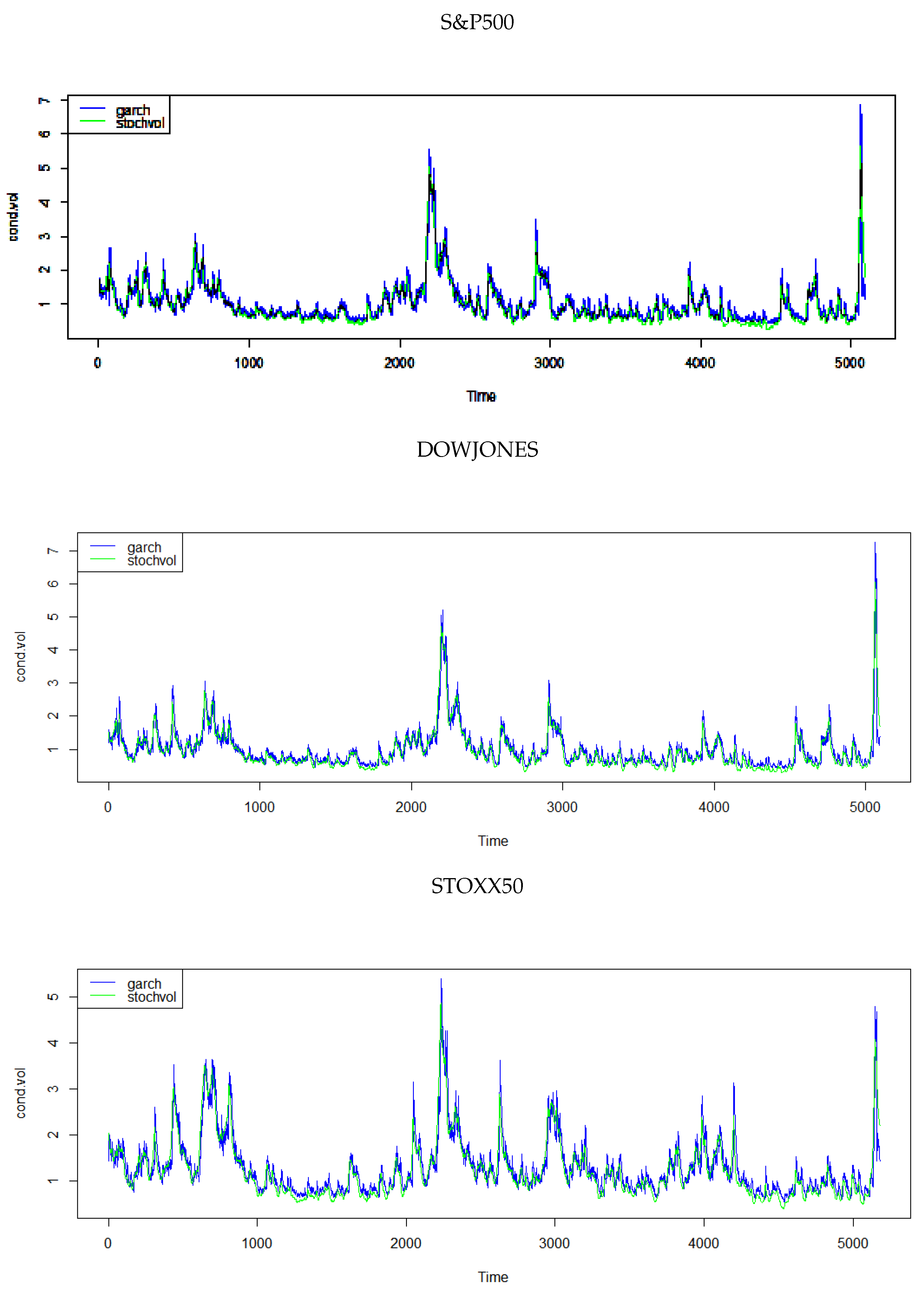
Figure 5. Mincer–Zarnowitz rolling regression slope coefficients bounded by two standard deviations.

Figure 5. Mincer–Zarnowitz rolling regression slope coefficients bounded past ii standard deviations.

Effigy 6. Posterior density plots of parameters in

$\theta$

.

Figure 6. Posterior density plots of parameters in

$\theta$

.

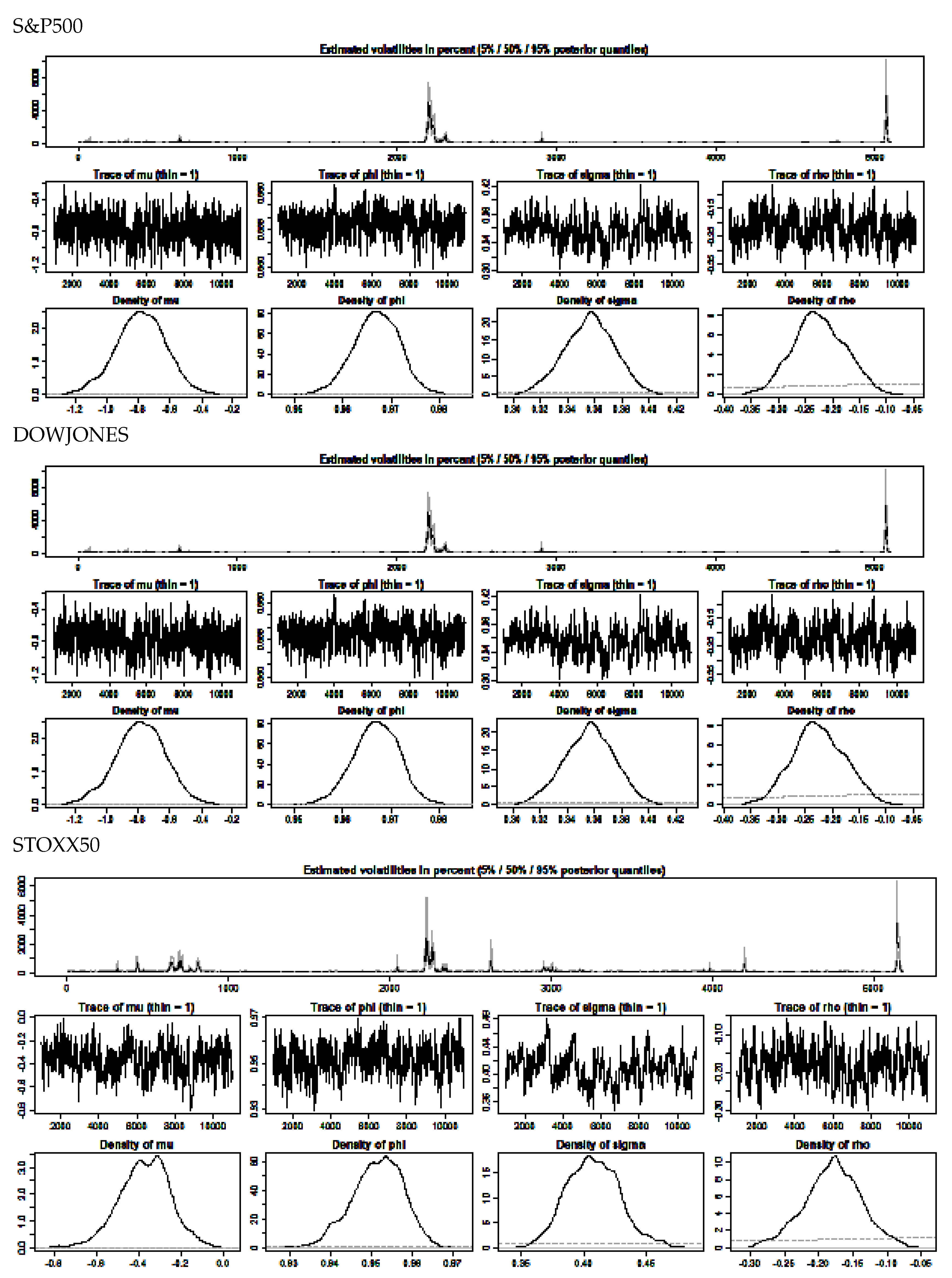
Table 1. Summary statistics.

Table 1. Summary statistics.

	Mean	Median	Minimum	Maximum	Standard Deviation	Skewness	Excess Kurtosis
SPRET	0.000136	0.000540	−0.126700	0.106420	0.012485	−0.360540	10.874
SPRV5	0.000112	0.000047	0.000001	0.007748	0.000269	ten.6520	188.60
DJRET	0.000150	0.000488	−0.138070	0.107540	0.011946	−0.376640	13.380
DJRV5	0.000114	0.000049	0.000001	0.008624	0.000287	12.0870	238.02
STOXX50RET	−0.000098	0.000236	−0.120050	0.105540	0.014399	−0.225470	5.8411
STOXX50RV5	0.000161	0.000081	0.000000	0.010827	0.000336	12.0260	256.24
Key:
SPRET	Continuously compounded close to close render on the South&P500 Alphabetize
SPRV5	Daily realised volatility on the S&P500 Index sampled at 5 min intervals provided by Oxford Human
DJRET	Continuously compounded close to close return on the DOWJONES Index
DJRV5	Daily realised volatility on the S&P500 Index sampled at five min intervals provided by Oxford Homo
STOXX50RET	Continuously compounded close to close return on the South&P500 Alphabetize
STOXX50RV5	Daily realised volatility on the Southward&P500 Index sampled at 5 min intervals provided by Oxford Man

Table 2. Stochastic volatility estimates.

Table 2. Stochastic volatility estimates.

Summary of 1000 MCMC Draws later Burn down in of 1000
Prior Distributions
$\mu \sim nor\mathrm{chiliad}al$	hateful = 0	S.D. = 100
$(\varphi +\mathrm{ane})/2\sim \beta$	$a_0=5$	$b_0=1.5$
${\sigma }^2\sim {\chi }^2(df=\mathrm{ane})$
Southward&P500
Posterior draws thinning = 1
	Mean	S.D.	v%	l%	95%
$\mu$	−9.4565	0.15973	−ix.7172	−9.4562	−9.193
$\varphi$	0.9803	0.00377	0.9739	0.9804	0.986
$\sigma$	0.2154	0.01526	0.1902	0.2152	0.241
$exp(\mu /\mathrm{two})$	0.0089	0.00071	0.0078	0.0088	0.010
${\sigma }^2$	0.0466	0.00659	0.0362	0.0463	0.058
DOWJONES
Posterior draws thinning = 1
	Mean	Southward.D.	5%	l%	95%
$\mu$	−9.5491	0.14899	−9.7890	−ix.7890	−9.3053
$\varphi$	0.9784	0.00393	0.9718	0.9785	0.9846
$\sigma$	0.2222	0.01509	0.1982	0.2214	0.2470
$exp(\mu /2)$	0.0085	0.00063	0.0075	0.0084	0.0095
${\sigma }^2$	0.0496	0.00676	0.0393	0.0490	0.0610
STOXX50
Posterior draws thinning = 1
	Mean	Due south.D.	5%	fifty%	95%
$\mu$	−8.969	0.15544	−nine.2223	−eight.969	−8.719
$\varphi$	0.983	0.00346	0.9774	0.983	−eight.719
$\sigma$	0.177	0.01362	0.1556	0.176	0.200
$e\mathrm{ten}p(\mu /2)$	0.011	0.00088	0.0099	0.011	0.200
${\sigma }^{\mathrm{two}}$	0.031	0.00484	0.0242	0.031	0.040

Table 3. GARCH(one,1) fitted to INDICES RETURNS.

Table three. GARCH(1,ane) fitted to INDICES RETURNS.

	Coefficients	Standard Error	T Statistic
South&P500
$\mu$	0.00071466	0.0001000	vii.144 ***
$\omega$	0.0000013037	0.0000002911	4.479 ***
${\alpha }_1$	0.12429	0.0118	10.530 ***
${\beta }_{\mathrm{one}}$	0.87470	0.01081	fourscore.918 ***
DOWJONES
$\mu$	0.00028945	0.0001063	2.723 ***
$\omega$	0.000001861	0.000000258	7.212 ***
${\alpha }_1$	0.12121	0.009328	12.995 ***
${\beta }_1$	0.86583	000.9399	92.123 ***
STOXX50
$\mu$	0.000093821	0.0001411	0.665
$\omega$	0.0000024108	0.000000407	5.911 ***
${\alpha }_{\mathrm{one}}$	0.099385	0.008582	11.580 ***
${\beta }_{\mathrm{one}}$	0.89020	0.009059	98.266 ***

Tabular array 4. Regression analysis of the three volatility models as Explanators of RV5.

Table iv. Regression analysis of the three volatility models as Explanators of RV5.

S&P500
OLS, using observations 2000-01-06–2020-04-xxx (T = 5098)
Dependent variable: rv5
	Coefficient	Std. Error	t-ratio	p-value
const	−0.000193903	4.80241 × 10${}^{-\mathrm{half\; dozen}}$	−twoscore.38	0.0000
STVOL_1	0.000305766	4.04560 × x${}^{-6}$	75.58	0.0000
Mean dependent var	0.000112	S.D. dependent var	0.000269
Sum squared resid	0.000174	South.E. of regression	0.000185
$R^{\mathrm{two}}$	0.528511	Adjusted $R^2$		0.528418
$F(1,5096)$	5712.306	P-value(F)		0.000000
$\widehat{\rho }$	0.355673	Durbin–Watson		1.288578
OLS, using observations 2000-01-06–2020-04-30 (T = 5098)
Dependent variable: rv5
	Coefficient	Std. Error	t-ratio	p-value
const	−0.000186320	v.58228 × 10${}^{-\mathrm{vi}}$	−33.38	0.0000
garchh_t_1	0.000282384	iv.54881 × 10${}^{-6}$	62.08	0.0000
Hateful dependent var	0.000112	S.D. dependent var		0.000269
Sum squared resid	0.000210	S.E. of regression		0.000203
$R^2$	0.430599	Adjusted $R^2$		0.430488
$F(\mathrm{i},5096)$	3853.762	P-value(F)		0.000000
$\widehat{\rho }$	0.432641	Durbin–Watson		i.134608
OLS, using observations 2000-02-02–2020-04-30 (T = 5079)
Dependent variable: rv5
	Coefficient	Std. Error	t-ratio	p-value
const	3.02687 × ten${}^{-5}$	2.84918 × 10${}^{-6}$	ten.62	0.0000
sq_DMSPRET_1	0.174138	0.00556030	31.32	0.0000
sq_DMSPRET_2	0.0933966	0.00559548	16.69	0.0000
sq_DMSPRET_3	0.0527851	0.00588575	viii.968	0.0000
sq_DMSPRET_4	0.0280498	0.00588689	4.765	0.0000
sq_DMSPRET_5	0.0591621	0.00588274	10.06	0.0000
sq_DMSPRET_6	0.0387770	0.00590617	6.565	0.0000
sq_DMSPRET_7	0.0127639	0.00593373	2.151	0.0315
sq_DMSPRET_8	0.0128494	0.00591714	2.172	0.0299
sq_DMSPRET_9	0.0460289	0.00591518	7.781	0.0000
sq_DMSPRET_10	0.0108100	0.00588990	1.835	0.0665
sq_DMSPRET_11	−0.0125045	0.00589057	−2.123	0.0338
sq_DMSPRET_12	0.00683578	0.00591643	1.155	0.2480
sq_DMSPRET_13	0.000837936	0.00591795	0.1416	0.8874
sq_DMSPRET_14	−0.00804767	0.00593584	−i.356	0.1752
sq_DMSPRET_15	−0.00239430	0.00590724	−0.4053	0.6853
sq_DMSPRET_16	−0.0108916	0.00588602	−ane.850	0.0643
sq_DMSPRET_17	0.00482912	0.00588926	0.8200	0.4123
sq_DMSPRET_18	0.0125097	0.00593287	2.109	0.0350
sq_DMSPRET_19	0.0123520	0.00564065	2.190	0.0286
sq_DMSPRET_20	−0.00717624	0.00560040	−1.281	0.2001
Mean dependent var	0.000112	Due south.D. dependent var		0.000269
Sum squared resid	0.000169	S.Eastward. of regression		0.000183
$R^{\mathrm{two}}$	0.541977	Adjusted $R^{\mathrm{two}}$		0.540166
$F(20,5058)$	299.2563	P-value(F)		0.000000
$\widehat{\rho }$	0.283092	Durbin–Watson		ane.433782
OLS, using observations 2000-01-06–2020-04-30 (T = 5094)
Dependent variable: rv5
	Coefficient	Std. Error	t-ratio	p-value
const	−0.000198625	five.37151 × x${}^{-\mathrm{six}}$	−36.98	0.0000
SVDJ_1	0.000328020	4.75466 × 10${}^{-6}$	68.99	0.0000
Hateful dependent var	0.000114	S.D. dependent var		0.000287
Sum squared resid	0.000216	S.Eastward. of regression		0.000206
$R^2$	0.483125	Adjusted $R^2$		0.483024
$F(1,5092)$	4759.515	P-value(F)		0.000000
$\widehat{\rho }$	0.331936	Durbin–Watson		ane.336075
OLS, using observations 2000-01-06–2020-04-xxx (T = 5094)
Dependent variable: rv5
	Coefficient	Std. Error	t-ratio	p-value
const	−0.000170947	6.16017 × ten${}^{-6}$	−27.75	0.0000
Djht_1	0.000280420	5.18265 × 10${}^{-\mathrm{six}}$	54.xi	0.0000
Mean dependent var	0.000114	S.D. dependent var		0.000287
Sum squared resid	0.000266	Southward.E. of regression		0.000228
$R^2$	0.365056	Adjusted $R^2$		0.364932
$F(1,5092)$	2927.610	p-value(F)		0.000000
$\widehat{\rho }$	0.434841	Durbin–Watson		ane.130290
OLS, using observations 2000-01-04–2020-04-30 (T = 5075)
Dependent variable: lrv5
	Coefficient	Std. Error	t-ratio	p-value
const	0.0405870	0.00329492	12.32	0.0000
SQDMDJRET_1	0.000165523	6.55973 × 10${}^{-6}$	25.23	0.0000
SQDMDJRET_2	0.000101750	6.61717 × ten${}^{-6}$	fifteen.38	0.0000
SQDMDJRET_3	5.22487 × x${}^{-5}$	6.99793 × ten${}^{-6}$	7.466	0.0000
SQDMDJRET_4	two.10587 × x${}^{-5}$	vi.99864 × ten${}^{-6}$	3.009	0.0026
SQDMDJRET_5	6.58804 × 10${}^{-5}$	7.00022 × 10${}^{-\mathrm{half\; dozen}}$	9.411	0.0000
SQDMDJRET_6	iv.64120 × 10${}^{-5}$	7.00145 × 10${}^{-6}$	6.629	0.0000
SQDMDJRET_7	1.56715 × 10${}^{-6}$	7.13269 × ten${}^{-6}$	0.2197	0.8261
SQDMDJRET_8	1.54284 × ten${}^{-\mathrm{six}}$	7.11737 × 10${}^{-6}$	0.2168	0.8284
SQDMDJRET_9	4.60489 × 10${}^{-5}$	vii.11644 × ten${}^{-\mathrm{six}}$	6.471	0.0000
SQDMDJRET_10	−ii.98185 × 10${}^{-6}$	seven.06670 × ten${}^{-\mathrm{vi}}$	−0.4220	0.6731
SQDMDJRET_11	−ane.35137 × 10${}^{-5}$	7.06710 × 10${}^{-\mathrm{vi}}$	−one.912	0.0559
SQDMDJRET_12	−2.77575 × 10${}^{-6}$	vii.11818 × x${}^{-6}$	−0.3900	0.6966
SQDMDJRET_13	5.94860 × ten${}^{-6}$	7.11930 × 10${}^{-6}$	0.8356	0.4034
SQDMDJRET_14	−8.20421 × 10${}^{-6}$	7.13518 × 10${}^{-6}$	−1.150	0.2503
SQDMDJRET_15	−8.26171 × x${}^{-\mathrm{half\; dozen}}$	seven.00344 × 10${}^{-\mathrm{half\; dozen}}$	−i.180	0.2382
SQDMDJRET_16	−4.30980 × ten${}^{-\mathrm{six}}$	7.00422 × 10${}^{-\mathrm{half-dozen}}$	−0.6153	0.5384
SQDMDJRET_17	vi.42163 × 10${}^{-\mathrm{six}}$	7.00281 × 10${}^{-\mathrm{half-dozen}}$	0.9170	0.3592
SQDMDJRET_18	2.34879 × 10${}^{-\mathrm{v}}$	vii.08619 × 10${}^{-6}$	3.315	0.0009
SQDMDJRET_19	2.02923 × 10${}^{-5}$	6.69703 × ten${}^{-\mathrm{half-dozen}}$	3.030	0.0025
SQDMDJRET_20	−4.02896 × ten${}^{-6}$	6.63951 × ten${}^{-6}$	−0.6068	0.5440
Mean dependent var	0.113763	S.D. dependent var		0.287164
Sum squared resid	230.9808	S.E. of regression		0.213782
$R^2$	0.447966	Adjusted $R^2$		0.445781
$F(20,5054)$	205.0615	p-value(F)		0.000000
$\widehat{\rho }$	0.324610	Durbin–Watson		1.350773
OLS, using observations 2000-01-06–2020-04-30 (T = 5179)
Dependent variable: rv5
	Coefficient	Std. Fault	t-ratio	p-value
const	−0.000255606	seven.97034 × 10${}^{-6}$	−32.07	0.0000
STOXXSV_1	0.000249773	4.26226 × ten${}^{-\mathrm{half\; dozen}}$	58.60	0.0000
Hateful dependent var	0.000161	S.D. dependent var		0.000336
Sum squared resid	0.000351	Southward.E. of regression		0.000260
$R^2$	0.398798	Adjusted $R^{\mathrm{ii}}$		0.398682
$F(\mathrm{one},5177)$	3434.088	p-value(F)		0.000000
$\widehat{\rho }$	0.334086	Durbin–Watson		1.331768
OLS, using observations 2000-01-05–2020-04-30 (T = 5179)
Dependent variable: rv5
	Coefficient	Std. Error	t-ratio	p-value
const	−3.19171 × x${}^{-6}$	4.70679 × 10${}^{-\mathrm{half-dozen}}$	−0.6781	0.4977
h2STOXX50_1	0.783757	0.0140212	55.90	0.0000
Hateful dependent var	0.000161	Southward.D. dependent var		0.000336
Sum squared resid	0.000364	S.E. of regression		0.000265
$R^{\mathrm{ii}}$	0.376384	Adjusted $R^2$		0.376264
$F(1,5177)$	3124.586	p-value(F)		0.000000
$\widehat{\rho }$	0.342843	Durbin–Watson		1.314043
OLS, using observations 2000-02-02–2020-04-30 (T = 5160)
Dependent variable: rv5
	Coefficient	Std. Error	ct-ratio	p-value
const	2.05927 × x${}^{-5}$	4.29557 × 10${}^{-6}$	4.794	0.0000
sq_DMSTOXXRET_1	0.118968	0.00666728	17.84	0.0000
sq_DMSTOXXRET_2	0.120534	0.00666684	18.08	0.0000
sq_DMSTOXXRET_3	0.0933684	0.00669582	thirteen.94	0.0000
sq_DMSTOXXRET_4	0.0896290	0.00678649	xiii.21	0.0000
sq_DMSTOXXRET_5	0.0342222	0.00682410	v.015	0.0000
sq_DMSTOXXRET_6	0.0105941	0.00684945	1.547	0.1220
sq_DMSTOXXRET_7	0.0193777	0.00684880	2.829	0.0047
sq_DMSTOXXRET_8	0.0415985	0.00685618	6.067	0.0000
sq_DMSTOXXRET_9	0.0676568	0.00686950	9.849	0.0000
sq_DMSTOXXRET_10	0.0648663	0.00687561	9.434	0.0000
sq_DMSTOXXRET_11	0.00745897	0.00687600	1.085	0.2781
sq_DMSTOXXRET_12	0.00363238	0.00687086	0.5287	0.5971
sq_DMSTOXXRET_13	0.00415015	0.00685846	0.6051	0.5451
sq_DMSTOXXRET_14	0.00309319	0.00685311	0.4514	0.6518
sq_DMSTOXXRET_15	0.0459385	0.00685415	half dozen.702	0.0000
sq_DMSTOXXRET_16	−0.0110292	0.00682975	−ane.615	0.1064
sq_DMSTOXXRET_17	3.58184 × x${}^{-\mathrm{five}}$	0.00680192	0.005266	0.9958
sq_DMSTOXXRET_18	−0.0226702	0.00671209	−iii.378	0.0007
sq_DMSTOXXRET_19	0.00604883	0.00668237	0.9052	0.3654
sq_DMSTOXXRET_20	−0.0196779	0.00668193	−ii.945	0.0032
Hateful dependent var	0.000161	S.D. dependent var		0.000336
Sum squared resid	0.000324	S.Due east. of regression		0.000251
$R^2$	0.445202	Adjusted $R^{\mathrm{two}}$		0.443043
$F(20,5139)$	206.1915	p-value(F)	0.000000
$\widehat{\rho }$	0.216381	Durbin–Watson		1.567234

Table v. Mincer–Zarnowitz regressions.

Table 5. Mincer–Zarnowitz regressions.

Method	Exam Statistic	Probability
S&P500
STOCHVOL	1.06838 × ten${}^{11}$	0.0
GARCH	1.01522 × 10${}^{\mathrm{eleven}}$	0.0
sq_DMSPRET-1	2205.89	0.0
DOWJONES
STOCHVOL	7.72384 × 10${}^{10}$	0.0
GARCH	7.33155 × 10${}^{\mathrm{ten}}$	0.0
sq_DMDJRET-ane	ane.84768 × x${}^{16}$	0.0
STOXX50
STOCHVOL	626.635	0.0
GARCH	2.7139 × x${}^7$	0.0
sq_DMSTOXRET-1	5449.58	0.0

Tabular array vi. Stochastic volatility estimates augmented SV model.

Table half-dozen. Stochastic volatility estimates augmented SV model.

Summary of 1000 MCMC draws after fire in of 1000
Prior Distributions
$\mu \sim normal$	mean = 0	S.D. = 100
$(\varphi +1)/2\sim \beta$	$a_0=5$	$b_0=\mathrm{1.five}$
${\sigma }^{\mathrm{ii}}\sim {\chi }^{\mathrm{ii}}(df=1)$
S&P500
Posterior draws thinning = 1
	Hateful	Southward.D.	5%	50%	95%
$\mu$	−0.78	0.1562	−ane.05	−0.78	−0.53
$\varphi$	0.97	0.0048	0.96	0.97	0.97
$\sigma$	0.36	0.0182	0.32	0.36	0.39
$e\mathrm{10}p(\mu /2)$	0.68	0.0529	0.59	0.68	0.77
${\sigma }^2$	0.13	0.0130	0.11	0.13	0.15
DOWJONES
Posterior draws thinning = 1
	Mean	S.D.	5%	50%	95%
$\mu$	−0.907	0.1447	−ane.14	−0.913	−0.656
$\varphi$	0.957	0.0058	0.95	0.957	0.966
$\sigma$	0.437	0.0232	0.40	0.435	0.478
$\mathrm{due\; east}\mathrm{ten}p(\mu /\mathrm{two})$	0.637	0.0462	0.56	0.634	0.720
${\sigma }^{\mathrm{ii}}$	0.191	0.0204	0.16	0.189	0.229
STOXX50
Posterior draws thinning = one
	Mean	South.D.	5%	50%	95%
$\mu$	−0.37	0.1197	−0.57	−0.37	−0.18
$\varphi$	0.95	0.0062	0.94	0.95	0.96
$\sigma$	0.41	0.0211	0.37	0.41	0.44
$exp(\mu /2)$	0.83	0.0494	0.75	0.83	0.92
${\sigma }^2$	0.17	0.0173	0.14	0.17	0.20

Tabular array 7. Regression assay of the iii augmented stochastic volatility and GARCH models as explanators of RV5.

Tabular array 7. Regression analysis of the three augmented stochastic volatility and GARCH models as explanators of RV5.

S&P500
OLS, using observations 2000-01-05–2020-04-30 (T = 5098)
Dependent variable: rv5
	Coefficient	Std. Error	t-ratio	p-value
const	4.80570 × 10${}^{-5}$	2.59906 × 10${}^{-6}$	18.49	0.0000
SVREGSPRET_1	five.61407 × 10${}^{-7}$	6.87701 × ten${}^{-\mathrm{ix}}$	81.64	0.0000
Mean dependent var	0.000112	S.D. dependent var		0.000269
Sum squared resid	0.000160	S.E. of regression		0.000177
$R^2$	0.566679	Adjusted $R^2$		0.566594
$F(1,5096)$	6664.347	p-value(F)		0.000000
$\widehat{\rho }$	0.288688	Durbin–Watson		one.422414
OLS, using observations 2000-01-05–2020-04-30 (T = 5098)
Dependent variable: rv5
	Coefficient	Std. Error	t-ratio	p-value
const	0.000136717	3.02817 × 10${}^{-6}$	45.xv	0.0000
yhat3_1	−0.0810177	0.00148855	−54.43	0.0000
Mean dependent var	0.000112	S.D. dependent var		0.000269
Sum squared resid	0.000233	Due south.E. of regression		0.000214
$R^2$	0.367610	Adjusted $R^2$		0.367486
$F(1,5096)$	2962.324	p-value(F)		0.000000
$\widehat{\rho }$	0.248686	Durbin–Watson		1.502451
DOWJONES
OLS, using observations 2000-01-05–2020-04-30 (T = 5094)
Dependent variable: rv5
	Coefficient	Std. Fault	t-ratio	p-value
const	7.08759 × ten${}^{-\mathrm{v}}$	3.11272 × 10${}^{-6}$	22.77	0.0000
DJSVREG_1	three.42022 × 10${}^{-7}$	5.52569 × 10${}^{-9}$	61.90	0.0000
Mean dependent var	0.000114	S.D. dependent var		0.000287
Sum squared resid	0.000239	Due south.East. of regression		0.000217
$R^{\mathrm{two}}$	0.429352	Adjusted $R^2$		0.429240
$F(1,5092)$	3831.187	p-value(F)	0.000000
$\widehat{\rho }$	0.382376	Durbin–Watson		1.235179
OLS, using observations 2000-01-06–2020-04-30 (T = 5093)
Dependent variable: rv5
	Coefficient	Std. Error	t-ratio	p-value
const	0.000144841	2.96368 × x${}^{-\mathrm{six}}$	48.87	0.0000
yhat7_1	−0.00213366	3.18142 × 10${}^{-5}$	−67.07	0.0000
Hateful dependent var	0.000114	Southward.D. dependent var		0.000287
Sum squared resid	0.000222	South.Eastward. of regression		0.000209
$R^2$	0.469072	Adjusted $R^2$		0.468968
$F(1,5091)$	4497.872	p-value(F)		0.000000
$\widehat{\rho }$	0.347045	Durbin–Watson		ane.305745
OLS, using observations 2000-01-05–2020-04-30 (T = 5179)
Dependent variable: rv5
	Coefficient	Std. Mistake	t-ratio	p-value
const	3.92593 × 10${}^{-\mathrm{v}}$	3.84434 × 10${}^{-6}$	10.21	0.0000
STOXXREGFAC_1	one.04919 × 10${}^{-\mathrm{half\; dozen}}$	1.55219 × 10${}^{-\mathrm{eight}}$	67.59	0.0000
Hateful dependent var	0.000161	Southward.D. dependent var		0.000336
Sum squared resid	0.000310	S.Due east. of regression		0.000245
$R^2$	0.468805	Adjusted $R^2$		0.468702
$F(1,5177)$	4568.947	p-value(F)		0.000000
$\widehat{\rho }$	0.212647	Durbin–Watson		1.574424
OLS, using observations 2000-01-05–2020-04-30 (T = 5179)
Dependent variable: rv5
	Coefficient	Std. Mistake	t-ratio	p-value
const	0.000191985	4.32834 × 10${}^{-6}$	44.36	0.0000
yhat2_1	−0.111512	0.00332039	−33.58	0.0000
Mean dependent var	0.000161	S.D. dependent var		0.000336
Sum squared resid	0.000479	S.E. of regression		0.000304
$R^2$	0.178889	Adjusted $R^2$		0.178731
$F(\mathrm{ane},5177)$	1127.876	p-value(F)	vii.0 × 10${}^{-224}$
$\widehat{\rho }$	0.258795	Durbin–Watson		ane.482403

© 2020 by the author. Licensee MDPI, Basel, Switzerland. This article is an open admission article distributed under the terms and weather condition of the Creative Eatables Attribution (CC By) license (http://creativecommons.org/licenses/by/4.0/).

davisaffire.blogspot.com

Source: https://www.mdpi.com/1911-8074/13/9/202/htm